Newton's method

This post and others are heavily inspired by Goodfellow's Deep Learning book. Newton's method is just a smarter version of gradient descent. Let $J(\theta)$ be our cost function. Gradient descent follows the gradient directly downhill from the previous point:

$$\theta_k = \theta_{k-1} - \nabla J(\theta_{k-1}) \quad \text{SGD}$$

There's one problem. The direction pointing directly downhill changes as we move.

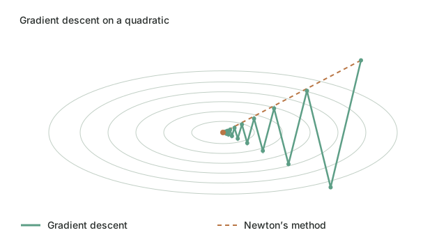
Newton's avoids this wasteful naivety by considering how the gradient will change as we move. Since the Hessian is the gradient of the gradient, we just left-multiply our step by the inverse Hessian:

$$\theta_k = \theta_{k-1} - H^{-1} \nabla J(\theta_{k-1}) \quad \text{Newton's}$$

So Newton's just rescales each element of the gradient by the weighted sum of its second derivatives. We can derive Newton's method with a few lines of calculus.

Taylor approximation

Remember that the Taylor polynomial approximates a function from the perspective of a given point. Here’s how successive Taylor polynomials approximate $\sin(x)$ around $x = 0$.

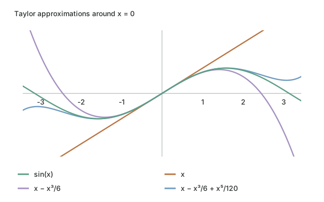
Well, it takes a lot of terms. You'll be surprised to hear that in a lot of optimization we only use two terms. Yeah, this is a bad approximation, but it works as long as we don't move too far. Besides, after we move, we'll make a new Taylor approximation from our new point, which will suit us for another small move from there.

Deriving Newton's from the Taylor expansion

If we look at the second-order Taylor polynomial from the perspective of $\theta_0$, we have

$$J(\theta_0) + (\theta - \theta_0) \nabla J(\theta_0) + \frac{1}{2} (\theta - \theta_0) H (\theta - \theta_0)^\top$$

This approximates our cost function $J(\theta)$, as long as we don't move too far from our perspective point $\theta_0$. Since we're trying to minimize our cost, we'll set its gradient equal to zero. That means, in one step, we'll move in the direction and distance that gets us to a flat gradient, assuming our quadratic approximation is accurate up until that point. This assumption can be good or bad. In deep learning it can end up jumping us to saddle points. A quick note: we're using column gradients below, so $(\theta - \theta_0)^\top$ is a row vector which forms a dot product with $J(\theta_0)$.

Finding the gradient

The gradient of the second-order Taylor approximation of the cost function is

$$\nabla \left[ J(\theta_0) + (\theta - \theta_0)^\top \nabla J(\theta_0) + \frac{1}{2} (\theta - \theta_0)^\top H (\theta - \theta_0) \right]$$

and by linearity of the gradient operator

$$\nabla J(\theta_0) + \nabla \left[ (\theta - \theta_0)^\top \nabla J(\theta_0) \right] + \frac{1}{2} \nabla \left[ (\theta - \theta_0)^\top H (\theta - \theta_0) \right]$$

The first term is zero since $\theta_0$ is fixed and we're taking the gradient with respect to $\theta$.

By linearity of transpose

$$\nabla \left[ (\theta^\top - \theta_0^\top) \nabla J(\theta_0) \right] + \frac{1}{2} \nabla \left[ (\theta^\top - \theta_0^\top) H (\theta - \theta_0) \right]$$

and linearity of matrix product

$$\nabla \left[ \theta^\top \nabla J(\theta_0) - \theta_0^\top \nabla J(\theta_0) \right] + \frac{1}{2} \nabla \left[ \theta^\top H (\theta - \theta_0) - \theta_0^\top H (\theta - \theta_0) \right]$$

and again upon the right side

$$\nabla \left[ \theta^\top \nabla J(\theta_0) - \theta_0^\top \nabla J(\theta_0) \right] + \frac{1}{2} \nabla \left[\theta^\top H \theta - \theta^\top H \theta_0 - \theta_0^\top H \theta + \theta_0^\top H \theta_0 \right]$$

Distributing and applying the gradient operators gives

$$\nabla J(\theta_0) + \frac{1}{2} \left[2 H \theta - H \theta_0 - (\theta_0^\top H)^\top + 0 \right]$$

and distributing the transpose across the product

$$\nabla J(\theta_0) + \frac{1}{2} \left[2 H \theta - H \theta_0 - H^ \top \theta_0 \right]$$

and exploiting the fact that the Hessian is symmetric such that $H^\top = H$

$$\begin{aligned} \nabla J(\theta_0) + \frac{1}{2} \left[2 H \theta - 2 H \theta_0 \right] \\[1.6em] \nabla J(\theta_0) + H(\theta - \theta_0) \end{aligned}$$

Setting the gradient to zero

So this is the gradient of our quadratic approximation of our cost function $J(\theta)$ when evaluated at our current parameter setting $\theta_0$. If we set this equation equal to zero and solve for $\theta$ we get the new parameter setting that sets our gradient equal to zero assuming that our quadratic approximation is valid up until that point:

$$\begin{aligned} \nabla J(\theta_0) + H(\theta - \theta_0) := 0 \\[1.6em] \nabla J(\theta_0) + H \theta - H \theta_0 = 0 \\[1.6em] H \theta = H \theta_0 - \nabla J(\theta_0) \\[1.6em] \theta = \theta_0 - H^{-1} \nabla J(\theta_0) \end{aligned}$$

Conclusion

Newton's method is gradient descent where we scale the gradient by the inverse Hessian. This gives Newton's foresight of how the gradient will change as we move, which lets us jump straight to the point where the gradient is zero if we so choose. A learning rate of $1$ will make this happen. A learning rate less than $1$ is more conservative.

Newton's has weakness. It will actually move uphill to a point of zero gradient, and that point could also be a saddle point rather than a local minimum. Additionally you have to use $O(n^2)$ operations to compute the Hessian. There are ways to fix these weaknesses, known as quasi-Newton methods. We'll explore these in future posts. $\quad \square$