Posted on June 25, 2017
A matrix-calculus approach to deriving the sensitivity of cross-entropy cost to the weighted input to a softmax output layer. We use row vectors and row gradients, since typical neural network formulations let columns correspond to features, and rows correspond to examples. This means that the input to our softmax layer is a row vector with a column for each class.
Softmax is a vector-to-vector transformation that turns a row vector
into a normalized row vector
The transformation is easiest to describe element-wise. The th output is a function of the entire input , and is given by
Softmax is nice because it turns into a probability distribution.
Softmax is invariant to additively scaling by a constant .
In other words, softmax only cares about the relative differences in the elements of . That means we can protect softmax from overflow by subtracting the maximum element of from every element of . This will also protect against underflow because the denominator will contain a sum of non-negative terms, one of which is .
def softmax(x):
    """Return the softmax of a vector x.

    :type x: ndarray
    :param x: vector input

    :returns: ndarray of same length as x
    """
    x = x - np.max(x)
    row_sum = np.sum(np.exp(x))
    return np.array([np.exp(x_i) / row_sum for x_i in x])
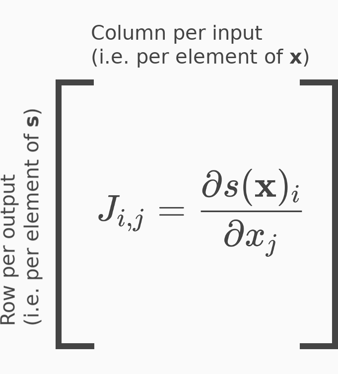
Since softmax is a vector-to-vector transformation, its derivative is a Jacobian matrix. The Jacobian has a row for each output element , and a column for each input element .
The entries of the Jacobian take two forms, one for the main diagonal entry, and one for every off-diagonal entry. We’ll show how to compute these entries for an arbitrary row of the Jacobian.
First compute the diagonal entry of row . That is, compute the derivative of the ‘th output, , with respect to its ‘th input, . All we need is the division rule from calculus.
Now compute every off-diagonal entry of row . That is, compute the derivative of the ‘th output, , with respect to its ‘th input, , where . Again we use the division rule, but in this case the derivative of the numerator, with respect to is zero, because means the numerator is constant with respect to .
This is nice! The derivative of softmax is always phrased in terms of softmax.
From now on, to keep things clear, we won’t write dependence on . Instead we’ll write as and as , understanding that and are each a function of the entire vector .
The form of the off-diagonals tells us that the Jacobian of softmax is a symmetric matrix. This is nice because symmetric matrices have great numeric and analytic properties. We expand it below. Each row is a gradient of one output element with respect to each of its input elements .
Notice that we can express this matrix as
where the second term is the outer product, because we defined as a row vector.
def jacobian_softmax(s):
    """Return the Jacobian matrix of softmax vector s.

    :type s: ndarray
    :param s: vector input

    :returns: ndarray of shape (len(s), len(s))
    """
    return np.diag(s) - np.outer(s, s)
Cross-entropy measures the difference between two probability distributions. We saw that is a distribution. The correct class is also a distribution if we encode it as a one-hot vector:
where the appears at the index of the correct class of this single example.
The cross-entropy between our predicted distribution over classes, , and the true distribution over classes, , is a scalar measure of their difference, which is perfect for a cost function. It’ll drive our softmax distribution toward the one-hot distribution. We can write this cost function as
which is the dot product since we’re using row vectors. This formula comes from information theory. It measures the information gained about our softmax distribution when we sample from our one-hot distribution.
def cross_entropy(y, s):
    """Return the cross-entropy of vectors y and s.

    :type y: ndarray
    :param y: one-hot vector encoding correct class

    :type s: ndarray
    :param s: softmax vector

    :returns: scalar cost
    """
    # Naively computes log(s_i) even when y_i = 0
    # return -y.dot(np.log(s))

    # Efficient, but assumes y is one-hot
    return -np.log(s[np.where(y)])
Since our is given and fixed, cross-entropy is a vector-to-scalar function of only our softmax distribution. That means it will have a gradient with respect to our softmax distribution. This vector-to-scalar cost function is actually made up of two steps: (1) a vector-to-vector element-wise and (2) a vector-to-scalar dot product. The vector-to-vector logarithm will have a Jacobian, but since it’s applied element-wise, the Jacobian will be diagonal, holding each elementwise derivative. The gradient of a dot product, being a linear operation, is just the vector .
where we used equation (69) of the matrix cookbook for the derivative of the dot product.
def gradient_cross_entropy(y, s):
    """Return the gradient of cross-entropy of vectors y and s.

    :type y: ndarray
    :param y: one-hot vector encoding correct class

    :type s: ndarray
    :param s: softmax vector

    :returns: ndarray of size len(s)
    """
    return -y / s
By the chain rule, the sensitivity of cost to the input to the softmax layer, , is given by a gradient-Jacobian product, each of which we’ve already computed:
The first term is the gradient of cross-entropy to softmax activation. The second term is the Jacobian of softmax activation to softmax input. Remember that we’re using row gradients - so this is a row vector times a matrix, resulting in a row vector. Expanding and simplifying, we get
The last line follows from the fact that was one-hot and applied to a matrix whose rows are identically our softmax distribution. But actually, any whose elements sum to would satisfy the same property. To be more specific, the equation above would hold not just for one-hot , but for any specifying a distribution over classes.
def error_softmax_input(y, s):
    """Return the sensitivity of cross-entropy cost to input of softmax.

    :type y: ndarray
    :param y: one-hot vector encoding correct class

    :type s: ndarray
    :param s: softmax vector

    :returns: ndarray of size len(s)
    """
    return s - y
Our work thus far considered a single example. Hence , our input to the softmax layer, was a row vector. Alternatively, if we feed forward a batch of examples, then contains a row vector for each example in the minibatch.
Softmax is still a vector-to-vector transformation, but it’s applied independently to each row of .
def batch_softmax(x):
    """Return matrix of row-wise softmax of x.

    :type x: ndarray
    :param x: row per example and column per feature

    :returns: ndarray of x.shape after row-wise softmax
    """
    # Stabilize by subtracting row max from each row
    row_maxes = np.max(x, axis=1)
    row_maxes = row_maxes[:, np.newaxis]  # for broadcasting
    x = x - row_maxes

    return np.array([softmax(row) for row in x])
Because rows are independently mapped, the Jacobian of row of with respect to row of is a zero matrix.
and the Jacobian of row of with respect to row of is our familiar matrix from before
That means our grand Jacobian of with respect to is a diagonal matrix of matrices, most of which are zero matrices:
def jacobian_batch_softmax(s):
    """Return array of row-wise Jacobians of s.

    :type s: ndarray
    :param s: matrix whose rows are softmaxed

    :returns: ndarray of shape
              (s.shape[0], s.shape[0], s.shape[1], s.shape[1])
    """
    # Array of nonzero Jacobians lying along tensor diagonal
    return np.array([jacobian_softmax(row) for row in s])
Let each row of be a one-hot label for an example:
Then we compute the mean cross-entropy by averaging the cross-entropy of every matching pair of rows of and . That is, we average over examples, the cross-entropy of each example:
The above simplification works because each row of is . So each column of is . So the matrix product dots rows of with columns of , which is exactly what we want for cross-entropy. Now, we only care about entries where the row index equals the column index. That’s because cross-entropy sums the dot products of matching rows of and . We can sum over matching dot products by using a trace.
Note: this formulation is computationally wasteful. We shouldn’t implement batch cross-entropy this way in a computer. We’re only using it for its analytic simplicity to work out the backpropogating error. However, the end analytic result is actually computationally efficient.
def mean_cross_entropy(y, s):
    """Return the mean row-wise cross-entropy of y and s.

    :type y: ndarray
    :param y: matrix whose rows are one-hot vectors encoding
              the correct class of each example.

    :type s: ndarray
    :param s: matrix whose every row is a softmax distribution over
              class predictions for a given example.

    :returns: scalar, mean row-wise cross-entropy cost
    """
    return np.mean([cross_entropy(y_row, s_row)
                    for y_row, s_row in zip(y, s)])
Since mean cross-entropy maps a matrix to a scalar, its Jacobian with respect to will be a matrix.
Since is an element-wise operation mapping a matrix to a matrix, its Jacobian is a matrix of element-wise derivatives which we chain rule by a Hadamard product, rather than by a dot product.
This procedure is always true for any element-wise operations. We can see this by concatenating the rows of .
such that is a row vector of length . Then is an element-wise vector-to-vector transformation again. So it has an diagonal Jacobian matrix.
If we flatten in the same way
then we get
and so
Now since and are each of length , we can reshape this formulation back into matrices, understanding that in both cases the division is element-wise:
and we have our result.
def jacobian_mean_cross_entropy(y, s):
    """Return the Jacobian matrix for mean cross-entropy.

    :type y: ndarray
    :param y: matrix whose rows are one-hot vectors encoding
              the correct class of each example.

    :type s: ndarray
    :param s: matrix whose every row is a softmax distribution over
              class predictions for a given example.

    :returns: ndarray of shape y.shape holding gradients as rows
    """
    return -(1 / y.shape[0]) * (y / s)
We apply the chain rule just as before. The only difference is that our gradient-Jacobian product is now a matrix-tensor product. Multiplying a matrix against a tensor is difficult. One approach is to flatten everything, do a vector-matrix product as before, and then reshape everything, but this is not elegant or intuitive. Instead, we dot rows of , each a gradient of a row-wise cross-entropy, against diagonal elements of , each a Jacobian matrix of a row-wise softmax.
We are able to do this because of the fact that is diagonal, which breaks the matrix-tensor product into an element-wise dot product of gradients and Jacobians. We owe this entirely to the fact that softmax is a row-to-row transformation, such that its Jacobian tensor is diagonal.
Where the third step followed by the fact that is diagonal. So the sensitivity of cost to the weighted input to our softmax layer is just the difference of our softmax matrix and our matrix of one-hot labels, where every element is divided by the number of examples in the batch.
def batch_error_softmax_input(y, s):
    """Return the sensitivity of cross-entropy cost to input of softmax.

    :type y: ndarray
    :param y: matrix whose rows are one-hot vectors encoding
              the correct class of each example.

    :type s: ndarray
    :param s: matrix whose every row is a softmax distribution over
              class predictions for a given example.

    :returns: ndarray of shape y.shape
    """
    return (1 / y.shape[0]) * (S - Y)